pODI Tutorial: Nonlinearity curve
This tutorial shows you how to create the nonlinearity cofficient file from a series of flat-fields with constant lamp setting and variable exposure time.
I like to have all my files sorted into subdirectories, so I usually put all raw files under raw/, all calibration files (bias, darks, flats, etc) under calib/ and all other science-y files in yet another directory. This scheme is implemented below, so if you organize your files differently you have to adjust the tutorial as needed.
First I create a directory to hold all files for this project, and then download/copy/link all needed raw files into the raw directory. For this tutorial I used a machine directly at WIYN, so I simply linked local copies of all files.
mkdir nonlinearity
cd nonlinearity
mkdir raw
cd raw
ln -s /mnt/odifile/archive/podi/TECH-13A-2003/2013.11.1?/[bdf]20* .
With all raw files in place, I’ll create a small log of all files that I can feed into the podi scripts.
~/bin/podi_svn+ssh/podi_getinfo.py $PWD/*/*33.fits > all.log
Now edit this file to only contain frames labeled “scp bias”, “scp dark” and all the files you need for the non-linearity curve (labeled “scp linearity”). Also make sure you don’t accidentally mix binned and unbinned frames. While collectcells can handle both cases, imcombine can’t handle these cases yet and you will likely run into some exception if you try to mix data binned differently. Save this file as nonlinearity.calib
On to creating the bias and dark files we need
cd ../
mkdir calib
cd calib
The non-linearity frames are domeflats, so we can’t simply run the usual podi_makecalibrations script. Instead, use the script to first create only the bias frame, and then only the dark frame. The -keeptemps option allows you to a) inspect the per-reduced individual files to make sure you only use the best files, and b) speed up reduction in case you find that one of the files in your stack really did screw things up.
~/bin/podi_svn+ssh/podi_makecalibrations.py ../raw/nonlinearity.calib . -only=bias -keeptemps
~/bin/podi_svn+ssh/podi_makecalibrations.py ../raw/nonlinearity.calib . -only=dark -keeptemps
Now on to creating the bias- and dark-subtracted frames:
cd ..
mkdir nonlin
cd nonlin
Again, edit the raw/all.log file and remove all bias and dark files, leaving only the domeflats that we need for the nonlinearity correction. I called this file nonlinearity.flats
We can now start the reduction of all these frames.
~/bin/podi_svn+ssh/podi_multicollect.py \
-fromfile=../raw/nonlinearity.flats \
-formatout=nonlin__%OBSID__%EXPTIME.fits \
-cals=../calib/
Depending on the number of CPU cores and the speed of your harddrive this process should only take a few minutes.
Measuring the intensity levels in all cells
The next step is to compute the average intensity levels for each cell in all the frames:
~/bin/podi_svn+ssh/podi_nonlinearity.py *.fits
This will create a small text file with all results. The file contains one line for each cell, with the following data in columns:
- OTA (e.g. 34)
- OTA-x (in the above case, this would be 3)
- OTA-y (and this 4)
- Cell-X
- Cell-Y
- Exposure time commanded (from header EXPTIME)
- Exposure time measured (from header EXPMEAS)
- Median Intensity in cell
- Mean intensity in cell
- Uncertainty of intensity
Only the OTA-X/Y, Cell-X/Y, commanded exposure time and median intensity will be used for the fit, the rest are left-overs from developing and for error checking.
Fitting the intensity-vs-time curves and computing the correction coefficients:
The last step is to create the actual coefficient fits. This is done via:
~/bin/podi_svn+ssh/podi_nonlinearity.py -fit nonlin.data coeffs.fits
The -fit option will run the actual fitting, nonlin.data is the data file with all the intensities that we created with the last command, and coeffs.fits is the output file. By default, the exposure times are limited to times between 0 seconds and 100 seconds and you most likely won’t have to change that. The other parameter is the intensity range used in the fit. You want the upper limit to be as high es possible (as the non-linearity effect becomes stronger at high intensity), but not saturated yet. During development, 59000 seemed to yield the most robust and reliable result.
Program execution will be fast, and spit out something like – it also prints the time and intensity levels used during the fit:
Creating all fits
 -----------------------------------------------------
 Polynomial order: 3
 Fit range exposure time [sec] = 0.000 - 100.000
 Fit range intensity [counts] = 10 - 59000
 -----------------------------------------------------
 Fitting OTA 61, cell 7,7 ...completed 819 fits
 done!
Create some diagnostic plots:
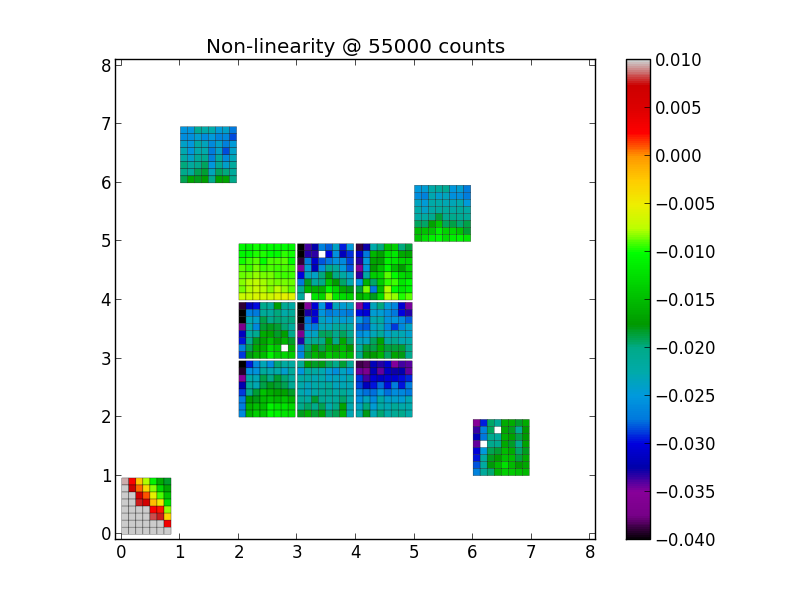
Now that we have all the coeffients, we might want to know the overall size of the non-linearity effect. The functionality to visualize the results is also in the pdi_nonlinearity.py file:
~/bin/podi_svn+ssh/podi_nonlinearity.py -nonlinmap coeffs.fits nonlinmap_user.png 55000 -min=-0.04 -max=0.01
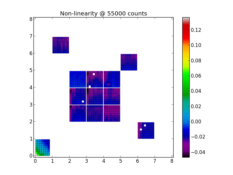
While convenient, the automatic scaling might not always be optimal to bring out more subtle differences. In this case, you can specify the minimum and maximum range directly on the command line, as done and shown below:
~/bin/podi_svn+ssh/podi_nonlinearity.py -nonlinmap coeffs.fits nonlinmap_user.png 55000 -min=-0.04 -max=0.01